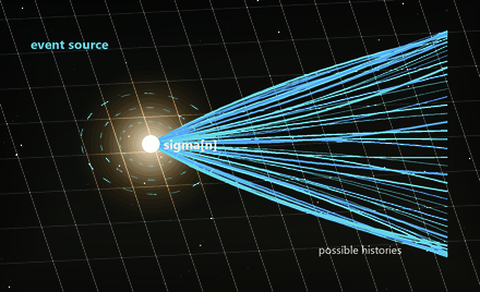
Central event
Look for the bright white centre labelled sigma[n]. This is the event being tested. The many rays show how many possible histories are being compared at once.
sigma[n] = (X[n], phi[n], mu[n], S[n])
S[n+1] = S[n] exp(-L[n] dt)
Each frame generates possible histories, tests them, then ranks what remains visible.
p_i = q_i G_i / sum(qG)
Reading the field
This first screen is a guided picture of the model. The bright glow is the event being inspected. The coloured rays are possible paths through the field. The three circles are moving bodies. The grid shows how the surrounding transport geometry is being bent. The small panels report which paths are still strong enough to count.
Start at the glow and follow the rays. A bright ray means that possible path is still well represented. A fading ray means it is losing weight as it passes through curvature, topology, closure pressure, or the moving bodies. The display is asking a simple question: out of all the possible paths, which ones survive this scene?
The colours give a quick reading of the path. Blue means the path is compressed or moving toward the observer in the effective-index view. Red means it is stretched, moving away, or entering a higher-index region. Violet and deeper colour mean the path is twisting as well as bending, so the line is carrying a torsion/z-depth cue rather than only a flat curve.
The three coloured bodies now run as a small live three-body solve. Their masses and positions change both the shape of nearby paths and the next orbital motion. Use Pause orbit to stop the bodies exactly where they are. Use Reset orbit to put just the bodies back at their starting phase. Use Restart sim when you want the whole scene and the right-hand controls returned to their defaults. The Object positions controls let you nudge the event, bodies, or merged black-hole centre and immediately see how the paths respond.
Light mode shows the paths travelling through the field. Wave mode redraws the same paths as a compact node view around the event, so you can compare the recursive classes without the ordinary rays filling the screen.
The density slider changes the visual support/mass scale used by this exploratory scene. Turn it high and the bodies move toward a merged black-hole-like bridge view. Near paths can lens around the centre; captured paths end there. Turn density the other way and the bodies behave like white-hole-like repulsive sources, sending matter-like fragments outward from the bodies themselves.
The black-hole and white-hole views are bridge sketches. They borrow familiar ideas like N-body inspiral, horizon growth, lensing, ringdown, repulsion, and frame dragging so the visual language can be explored, but this page is not claiming to derive a full astrophysical black-hole, white-hole, or loss law.
The merged black hole can be read two ways. Schwarzschild mode sets the
spin parameter a to zero, so the horizon is drawn without
frame dragging. Kerr mode gives the merged horizon non-zero spin and shows
the surrounding transport rings being dragged around it. Spin extraction
is a Penrose-style bridge sketch: imported pair-production and ergoregion
physics are drawn as a readable spin-drain story, with the escaping branch
carrying energy away and the displayed a relaxing toward zero.
Recovery assimilation adds the black-hole recovery note. It shows four zones at once: exterior paths that can still be reconstructed, a near-horizon processing layer, the horizon as the point where exterior recovery of the original carrier fails, and an interior support stack where conserved measure is added to the black-hole bookkeeping. The outgoing glow is drawn from the boundary layer, not from deep inside the hole, so it reads as radiation, jets, or ringdown rather than the same infalling photon escaping.
In Wave mode, n1, n2, n3, and
n4 are successive node classes along the same histories.
The ordinary light paths show where histories travel. The wave view
shows how those histories are grouped by the recursive update.
The background grid is the transport geometry. When curvature rises, the grid warps and the histories bend with it. The dotted rings are the observer-centred effective index/redshift bands. They help show lookback distance and changing propagation conditions.
The faint warm patches behind the lines are the exposure field. They mark regions where histories pay a higher survival cost because of curvature, interaction with the bodies, closure pressure, or active topology.
The square cell field is the Surtea topology layer. It now covers the
scene as a support partition rather than sitting off to the side. Each
body and the event carries its own local support object X[n].
Green cells are interior, red cells are boundary, and amber cells are
closure. Turning up topology heat makes the partition finer and more
unstable, so the boundary becomes more active.
Surtea-Austin bridge now reads as a working chain rather
than a badge. A support cell cluster splits into interior, boundary, and
closure regions. The boundary share becomes BD(X), which
modulates Gamma and therefore the visible survival weight of
the live histories. Phase exposure W stays separate.
The equation box is the recursive survival rule. L_eff is a
live loss score assembled from the current settings. Higher curvature,
stronger survival filtering, hotter topology, and stronger closure pressure
push it up. Coherence memory pulls it down by helping histories persist.
The recursive engine panel shows the actual loop being modelled:
histories are generated, transported, exposed to loss, filtered by
survival, passed through exposure-gate transmissions, and then renormalised into represented weights
p_i. In plain English: the panel asks "which possible paths
are still strong enough to count?" The bars show the five histories that
currently dominate the represented picture.
Recursive Survival Geometry treats observed structure as the persistence of
generated histories. The visual field begins with a structured state,
sigma[n] = (X[n], phi[n], mu[n], S[n]), and lets many possible
histories propagate outward. Bright paths are histories that retain survival
weight; fading paths are histories that lose coherence, closure, or
representation.
Curvature is drawn as a transport geometry rather than a pulling force.
Light-like modes remain open, low-loss, and non-closing. Matter-like
persistence appears where histories thicken, loop, or form records. Entropy
is the Shannon readout of the normalised survival measure: high
Hsurv means many survival-compatible histories remain live,
while low Hsurv means filtering has concentrated representation
into fewer basins.
The Surtea layer adds the topological foundation: support, interior, closure, boundary, class, and interaction. RSG explains how histories survive; Surtea explains what kind of support or object those histories are carried by.
The Surtea-Austin bridge is the bridge between those two ideas. It does
not say the gauge is the object. The object is still the carried support
X[n]. The visual reads the interior/boundary split, forms
BD(X), and lets that boundary share change the loss coefficient
while the ordinary RSG phase exposure remains visible as its own term.
Topology heat cools or warms the partition layer: cool cells are larger and stable, while hotter cells become finer, more restless, and more boundary-rich. Closure bias and coherence memory tune how readily light-like transport begins to form persistent records.
In the live readout, Hsurv = -sum p_i ln p_i is computed from the
survival-normalised path weights, and Nlive = exp(Hsurv) is the
effective number of represented histories. When survival loss keeps separating
the path family, the entropy-flow reading is dHsurv/dt = -Cov(A, Gamma W).
This interface is exploratory. It helps inspect path families, projection artefacts, numerical behaviour, and candidate analogue-test designs, but it is not itself validation data for RSG.
The first falsifiable target is a controlled analogue medium. In that
setting the update rule, path family, calibrated loss Γ,
exposure W, boundary conditions, detector response, output map,
and failure threshold have to be fixed before the output intensities are
compared.
The core test is whether accumulated survival loss
A = ∫ ΓW dt predicts measured logarithmic output
ratios better than ordinary attenuation ∫ Γ dt in a
declared positive-control regime.
Look for the bright white centre labelled sigma[n]. This is the event being tested. The many rays show how many possible histories are being compared at once.
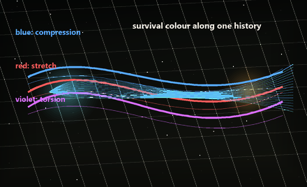
Follow one line rather than the whole bundle. Blue segments are compressed, red segments are stretched, and violet/deeper strokes mark twist along the path.
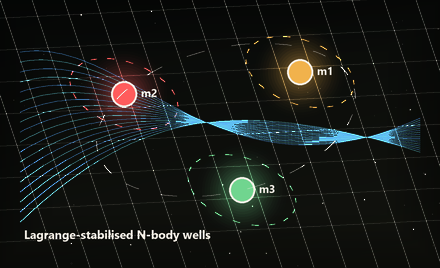
The amber, red, and green circles are live N-body wells. Their trails show the local motion from their current positions and velocities, while nearby histories bend, focus, or loop around them.
At high positive density the bodies coalesce into one horizon-like bridge view and the surrounding rings show frame dragging. At negative density, the bodies act as repulsive white-hole-like source sketches.
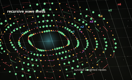
This is the same light history information redrawn as recursive wave layers. Green nodes are higher-survival represented points, red nodes are lower-survival points, blue marks strong compression, and amber marks captured nodes.
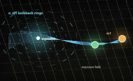
The dotted rings are effective-index/lookback guides. The soft coloured pressure behind the grid marks places where histories pay extra survival cost.
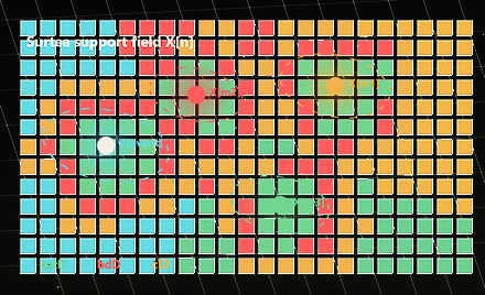
The square cells are the world-space topology layer beneath the smooth paths. Each body has a local Surtea support, while the full scene is divided into interior, boundary, and closure regions.
RSG is the basic field view: generated histories, survival weighting, live N-body wells, and represented paths.
Curvature makes the transport geometry easier to read, especially how the bodies and effective index bend light histories.
Entropy brings the Shannon readout of represented survival measure forward, so unresolved live alternatives and narrowing survival basins are easier to see.
Topology foregrounds Surtea's support layer, where cells mark interior, boundary, closure, and object support beneath the smooth paths. Surtea-Austin bridge turns that support layer into an operational chain: boundary exposure changes loss, and loss changes which histories remain represented. The preset strip is grouped by colour: core scenes, support scenes, measurement scenes, geometry scenes, render/light scenes, black-hole scenes, and external bridge scenes.
Bridge scenes such as black-hole, white-hole, spin extraction, recovery assimilation, and high-redshift views are future-application sketches. They are useful for comparison and intuition, while the present evidence claim belongs to a predeclared analogue-media test.
Presets jump to readable scenes in grouped sets of four. Each normal preset now gets a bottom-left card with a small schematic, a plain-English explanation of what the filter is showing, the active readout, and live gauges for the important quantities. Changing sliders keeps the chosen preset lit; the card button switches the gauges between the preset reference values and the current manual values. Preset info hides or shows these cards. The bridge presets keep their larger visual cards, with their purpose shown in both text and diagrams. Light-like keeps paths open and low-loss. Matter-like pushes closure and record-forming. Surtea partition shows the support layer beneath those histories. Surtea-Austin bridge shows BD(X) changing Gamma and survival. FFT spectrum turns a sampled trace into frequency bins, leakage, windows, and Nyquist limits. Vacuum support shows energy sites, relation vectors, support selection, boundary valuation, and conditional stress-energy contrast. Vopson bridge is an external comparator for information cost and compression, not a core RSG claim. Probability map separates preparation weight, accumulated loss, gate transmission, and represented output fraction. Analogue test shows the locked layered-medium comparison against ordinary attenuation. Surtea-Kelley shows boundary contact multiplied by recursive phase overlap. Angle-free Lorentz and No-angle torus show how unit vectors and closed update cycles can carry geometry without treating angles as primitive.
Recursion depth adds more update steps. Drag it right and the lines travel farther, so you see more bending, fading, looping, and long-range structure.
Curvature strengthens both the transport deformation and the live three-body coupling. Drag it right and the grid warps more strongly while the bodies pull on one another harder, so a manual position change becomes a new orbital condition rather than a cosmetic move.
Effective index increases the observer-centred propagation index. Drag it right and the dotted lookback rings become more important; distant histories slow visually and read as more redshifted. In the live paths, blue means a compressed or toward-observer segment, while red means a stretched or away/higher-index segment.
Survival filter raises the penalty for unstable histories. Drag it right and weak paths disappear faster, leaving fewer bright surviving bundles.
Topology heat controls the Surtea cell layer. Cool means larger, calmer cells with stable boundaries. Hot means smaller, twitchier cells with more active partition boundaries.
Surtea-Austin bridge uses topology heat as the partition-resolution control. Higher heat makes the boundary share larger, raises the visible BD(X) gauge, and lowers the survival bars when boundary exposure is doing more work.
Closure bias makes histories more willing to curl around the bodies. Drag it right and open light-like paths are pushed toward loops, thickening, and record-like behaviour.
Coherence memory gives surviving histories persistence from previous steps. Drag it right and coherent paths keep their shape longer instead of fading immediately.
Orbit speed now scales the physical three-body time step: positive evolves the N-body solve forward, negative steps it backward, and zero leaves the bodies still. Pause orbit freezes the bodies exactly where they are without changing that speed. Click it again to continue from the same positions and velocities. Reset orbit rebuilds a mass-weighted triangular Lagrange seed, with a light numerical stabiliser in ordinary planet mode so the browser demo stays in a readable orbit instead of drifting into escape. In merged black-hole presets, the speed value also reads as spin: zero is Schwarzschild-like, while non-zero speed gives a Kerr-like horizon with visible frame dragging. Simulation speed controls the whole recursive clock: negative values run the scene backward, zero freezes the clock, and positive values run it forward. Previous step and Next step pause the scene, light the main pause button, and move one scaled clock tick backward or forward.
Planet density scales effective mass/support strength and feeds into the orbit solver. High density increases attraction and moves the scene toward a black-hole-like capture/lensing bridge, with inspiral and ringdown drawn as standard-metric-inspired cues. Negative density opens a white-hole-like repulsive bridge and emits matter-like survival fragments from the white-hole bodies. Planet size changes the drawn radius without by itself increasing mass. Light display switches between ordinary light paths and a fixed event-centred wave view of light-node classes. Object positions lets you pick the event, bodies 1-3, or the BH centre and nudge it with the pan buttons; moving a body now changes the subsequent orbit. Throw random asteroid launches a small incoming body from a random edge and draws its survival path. Restart sim rewinds the recursive clock and restores the full right panel to its default light, density, size, and speed settings.
Recovery assimilation uses the same density and speed controls, but reads them as black-hole measure cues. Density sets the horizon/support scale; speed sets the spin term used by the boundary rings. The right-hand bars in the canvas are not detector values. They are visual handles for the conserved package M, J, Q, A_H: mass-energy, angular momentum, charge, and horizon area after the original carrier is no longer exterior-recoverable.
Filtered switches between raw generated histories and survival-weighted representation. Raw shows the candidates before selection; filtered shows what remains represented.
Labels names a few paths as open, near-closing, record-forming, or fading. n_eff bands turns the effective-index rings on or off. Surtea layer overlays the topology cells. Pause freezes the current recursive state so you can inspect it.
String waves draws the ordinary light histories as oscillating strings instead of straight segments. Wave recursions sets how many expanding node layers Wave mode draws: each n-layer is a torus-like wave shell carrying all sampled histories at that recursive step, coloured by survival weight and red/blue shift. Show objects only hides or shows the visible bodies/BH and their body trails; the hidden masses still bend the grid, lens the light, feed the wave view, and affect survival weight. Presets normally show objects, light, and non-wavy strings, but if you deselect Show objects, select Hide light, or turn on String waves, the following presets respect that choice until you switch it back. Hide light turns off the ordinary light histories and light-cone marks, which is also what Wave mode does by default so the node view can be read cleanly.
Peter M. Austin / RSG: Light-like, Matter-like, Entropy cloud, Three-body, and the base recursive survival engine.
Traian Surtea: Surtea partition, Surtea-Austin bridge, and the topology side of Matter-like, Layered stack, and Self-History Memory. Surtea-Austin is the bridge diagnostic: Surtea supplies interior/boundary/closure, while the added Austin valuation feeds boundary exposure into RSG survival loss.
FFT and vacuum support: FFT spectrum imports ordinary sampled-signal measurement language: time trace, bin spacing, windowing, leakage, and Nyquist limit. Vacuum support uses the vacuum-energy support note as a visual bridge from energy sites and relation vectors into support, valuation, and conditional stress-energy contrast.
Melvin M. Vopson / information comparator: Vopson bridge is included as an external comparison layer for information mass, Landauer cost, and infodynamic compression. It is deliberately labelled as speculative/comparator material; see mass-energy-information equivalence and computational-gravity listing.
Probability and locked analogue test: Probability map follows the RSG probability note: prepared amount q_i passes through G_i = exp(-A_i), then becomes p_i = q_iG_i / sum(qG). Analogue test keeps the empirical claim narrow: a fixed layered-medium setup must predict measured output and log-ratios before seeing the result, and it must beat ordinary attenuation in the declared positive-control case.
Surtea-Austin-Kelley phase compatibility: Surtea-Kelley adds Kelley's phase-compatibility layer to Surtea boundary support and Austin exposure weighting. The panel reads compatibility as boundary contact times phase overlap, meaning a cleaner recursive route, not a claim that ordinary spacetime distance has physically shrunk.
Angle-free Lorentz and no-angle torus: Angle-free Lorentz uses the corrected angle-free file. Direction is carried by unit vectors such as u_1 and u_2; the comparison is the Lorentzian invariant chi = alpha1 alpha2 - rho1 rho2 (u1.u2). No-angle torus extends the same idea to two closed unit cycles, U and V, so a closed recursive update can be read as one extended support object. Angles, rapidities, and torus parameters can be useful coordinates, but they are not primitive in these views.
Johann Pascher / FFGFT: FFGFT xi path, with links to redshift-as-path-stretch, xi-vacuum scale ladders, Casimir scale, and the static-cosmology/lithium sketches.
Paul Phillips / ZUOM: ZUOM lattice, treated as a computational conjecture layer for canonical filters, projection signatures, tower/lattice checks, and accepted/retracted artefacts.
George Moseley / ITR: ITR clock and High-z, where clock, update cost, saturation, and high-redshift maturation are imported as conditional substrate terms.
Emerson C. King / Render: Render map and the Render side of Pair threshold. The Render label is kept, but in this visual it is treated as an Einstein-Planck mass-frequency reformulation: E = hf and E = mc^2 imply m = hf / c^2. That is why the Render preset sits so close to Matter-like: frequency transport is being read as a mass-equivalent represented measure, while RSG still supplies the survival, closure, and support conditions. The pair threshold uses standard electron-positron threshold bookkeeping as an imported physics bridge, not as a derivation from RSG alone.
Jim Kelley / Kelley bridge: Kelley bridge is a correspondence-check preset for resonance, bridge constraints, and survival-filter consistency. It is included as a diagnostic bridge layer rather than a replacement for the RSG core.
Black-hole recovery / Recovery assimilation: Recovery assimilation follows the black-hole recovery note. It treats the horizon as a recovery boundary: original carrier history becomes unavailable to the exterior protocol, while projected conserved measure updates the black-hole package through processing and conservation maps. The interior support operator remains deliberately open.
Johann Pascher, Paul Phillips, Jim Kelley, and Isaid Rodriguez also sit in the broader bridge/correspondence ecology rather than replacing the RSG core.
exp(Hsurv).dHsurv/dt = -Cov(A, Gamma W).X[n] for an object or history.sigma[n] = (X[n], phi[n], mu[n], S[n]): support, phase/transport, measures, and survival weight.M_R = h f / c^2. In RSG it is a matter-like transport layer: frequency-energy has a mass-equivalent measure, but only becomes matter-like persistence when closure, support, recurrence, and survival weight are also present.2m_e c^2 = 1.022 MeV. In a two-photon head-on reading, each photon carries about 1.24 x 10^20 Hz.Surtea zoom
This is a frozen close-up of the Surtea layer from the live view. The
small squares are partition cells, or D-photons. A possible
object or event is carried by a support X[n], but the theory
does not read that support as a smooth blob first. It reads it through
interior, boundary, and closure.
In the RSG bridge, this matters because topology can affect survival. If a history keeps a stable support and stable boundary, it loses less weight. If its boundary shifts, its class changes, or it interacts through closure, it pays a higher survival cost.
The Surtea-Austin bridge preset turns this close-up into
a live operational view. It counts interior and boundary cells, turns the
boundary share into BD(X), and shows how that changes
Gamma, Lambda, and the surviving histories on
the canvas.
int_D(X): cells safely inside the support.bd_D(X): unstable edge where interaction and class change appear.cl_D(X): cells needed to close or complete the support.bd_D(X) = cl_D(X) - int_D(X)
RSG adds survival: stable boundary means lower loss; unstable partition change means higher loss.
Surtea topology and the new bridge layers
The new notes do not collapse everything into one claim. They stack the ideas. Surtea first defines what a support, interior, boundary, closure, class, and interaction can mean. RSG then asks which histories carried by those supports survive. The ITR and Render material are bridge layers: useful ways to attach clock, update cost, saturation, and frequency-mass bookkeeping without making those imports core RSG axioms.
The structured state is not only a moving dot. It is a package:
X[n] is the Surtea support, phi[n] is the
smooth transport projection, mu[n] stores physical
measures, and S[n] is the survival weight.
That is why the live canvas has both a smooth transport field and a square cell layer. The cells say what kind of object/support exists; the lines say which recursive histories remain represented.
The layered note also gives Surtea's self-history idea a place to live: a present support can remain coupled to its own previous supports through closure, boundary, or interaction.
In the visual language, this is the after-image of a cell object. Coherence memory makes those prior supports matter for longer, so a history resists sudden change and begins to feel more inertial.
Johann's FFGFT material can be shown as an optional
xi-vacuum overlay. In the visualisation, that means
path-stretch redshift: the light-like histories remain open, but
their effective length L_eff becomes longer than the
direct distance d.
The Casimir and redshift briefings also introduce a scale-ladder
reading: a single xi = 4/30000 is used to relate
redshift, Hubble-scale bookkeeping, and a claimed Casimir/CMB
scale. On this page, that belongs as a diagnostic overlay, not as
the base survival law.
The ZUOM architecture is best represented as a computational conjecture layer. Its own diagrams are about canonical matrices, projection landscapes, tower/lattice signatures, anchors, and explicit triage between verified and retracted artefacts.
In RSG terms, this does not need to become a new force or new geometry. It can sit as a pattern-testing surface over generated histories: which projections recur, which signatures survive, and which artefacts should be filtered out before they are treated as structure.
ITR is shown as a conditional substrate channel. It can add a candidate vacuum clock, Landauer update cost, and saturation factor to the ordinary RSG survival loss.
In page terms, the ITR clock preset raises the effective-index readout and filtering pressure. The key caution is that this is a bridge equation, not a claim that RSG requires the Moseley scale.
L = Gamma W + beta rho_I sigma(z) CThe high-redshift brief asks whether a saturation-limited update channel can make structure look mature early without allowing unlimited runaway processing.
Visually, this is represented as faster concentration of surviving
histories. The important diagnostics are not just "more structure",
but concentration C(z), closure persistence
B(z), and whether the saturated run stays between weak
baseline filtering and explosive unsaturated growth.
The Render note is best read as the Einstein-Planck
mass-frequency measure inside RSG: E = h f,
E = m c^2, therefore M_R = h f / c^2.
It is not photon rest mass and it is not a new constant. It is a
disciplined way to attach frequency-energy data to
mu[n].
That is why Render sits so close to matter-like closed transport: it already gives the frequency channel a mass-equivalent measure. RSG then supplies the hard part: when does that measured transport stay open and light-like, and when does it acquire closure-compatible support, recurrence, and survival weight so it reads as matter-like persistence?
In this page's language, Render is not "light becoming matter" by bookkeeping alone. It is the measure layer that becomes matter-like only when the surrounding RSG conditions close the transport into a persistent represented record.
The lightest matter-antimatter threshold is an electron and a
positron. The total energy needed is 1.022 MeV, which
is 2m_e c^2. A frequency of about
1.24 x 10^20 Hz corresponds to one electron rest
energy, m_e c^2 = 0.511 MeV.
So the clean visual reading is two high-frequency gamma channels
meeting head-on, each at about 1.24 x 10^20 Hz. If a
single photon supplies the full 1.022 MeV, the
equivalent frequency is about 2.47 x 10^20 Hz, and a
nearby field or nucleus must take recoil because one photon alone
cannot conserve momentum in empty space.
In RSG terms, matter-like persistence requires more than high
frequency. The light-like histories must also satisfy closure,
conservation, and support conditions so the energy becomes a
represented e- / e+ pair rather than remaining open
propagation.
Source library
The canvas is a visual guide to the document stack rather than a standalone simulation claim. The current framing treats this interface as exploratory; validation belongs to a predeclared analogue-media protocol. Each preset points back to a cluster of notes: core RSG definitions, probability, Surtea topology, light and propagation, entropy, early-structure modelling, correspondence layers, and source discipline texts.
The base visual language: generated histories, exposure-gate transmission, represented measure, locked analogue tests, three-body closure, and constrained early-structure modelling.
The cell overlay comes from the topological objecthood layer: support, interior, closure, boundary, class, interaction, and self-history memory, with both primary and simplified versions.
These notes anchor the light transport side: Maxwell field propagation, observer-centred effective index, redshift readouts, angle-free Lorentz embedding for coordinate time and linked support, and the threshold where high-frequency light can participate in matter-like pair production.
The fourth black-hole preset is a visual sketch rather than a link to a separate black-hole PDF. It treats the horizon as a recovery boundary: carrier identity is no longer exterior-readable, while conserved measure is shown as mass, spin, charge, area, and boundary bookkeeping. The vacuum-support note supplies the written guardrails for support-gated measure.
Probability is treated as normalised survival-representation weight; entropy is then read explicitly as Shannon scalar readout of that represented survival measure, with scalar and operator notes nearby.
ITR and conserved-sector notes are treated as conditional bridges: useful for update-cost and high-redshift maturation diagnostics, but not required as core RSG axioms.
These texts shape the surrounding craft: proportion, witness, field discipline, publishing format, and the careful translation of martial language into repair rather than conquest.